The “Gordon model” or viewing a stock as a bond with ever-increasing interest on coupons. Gordon's model and business valuation formula for investment or purchase Dividend growth rate per share
The Gordon model is used to estimate the cost of equity and profitability of ordinary shares. It is also called the constant growth dividend formula.
Since the growth of its value depends on the speed of increase in dividend payments of an enterprise. Let's look at the model formula in Excel using practical examples.
Gordon model: formula in Excel
The task of the model is to estimate the cost of equity, their profitability, and the discount rate for an investment project. Gordon's formula applies only in the following cases:
- the economic situation is stable;
- the discount rate is greater than the growth rate of dividend payments;
- the enterprise has sustainable growth (production and sales volume);
- the company freely accesses financial resources.
Formula for estimating return on equity using the Gordon model - calculation example:
r = D 1 /P 0 + g
- r – profitability of the enterprise’s own funds, discount rate;
- D1 – dividends in the next period;
- P0 – share price at this stage of the company’s development;
- g – average growth rate of dividend payments.
To find the size of dividends for the next period, they need to be increased by the average growth rate. The formula will look like:
r = (D 0 * (1 + g))/P 0 + g
Let's estimate the profitability of the shares of Mobile TeleSystems OJSC using the Gordon model. Let's draw up a table where the first column is the year of payment of dividends, the second is dividend payments in absolute terms.
Gordon's formula “works” under certain conditions. Therefore, first we check that the dividend values obey the exponential distribution law. Let's build a graph:
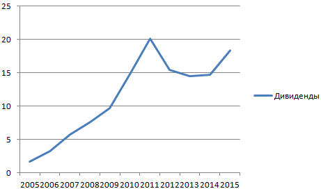
To check, add a trend line with the approximation reliability value. For this:


Now it is clearly visible that the data in the “Dividends” range obeys the exponential distribution law. Reliability – 77%.
Now we find out the current value of an ordinary share of Mobile TeleSystems OJSC. This is 215.50 rubles.
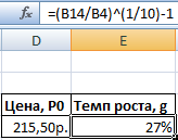

Thus, the expected return on the shares of Mobile TeleSystems OJSC is 38%.
Business valuation method based on the Gordon model in Excel
The value of an investment object at the beginning of the next period, according to the Gordon formula, is equal to the sum of current and all future annual cash flows. The amount of annual income is capitalized - the value of the business is formed. This is important to consider when assessing the value of a company.
Calculation of the capitalization rate using the Gordon model in Excel is carried out according to a simplified scheme:
FV = CF (1+n) / (DR – t)
The essence of the formula for estimating the value of a business is almost the same as in the case of calculating the future profitability of a stock. To determine the value of a business, slightly different indicators are taken:
- FV – the amount of equity capital;
- CF (1+n) – expected cash flows;
- DR – discount rate;
- t is the growth rate of cash flows in the residual period.
The difference in the denominator of the equation (DR – t) is called the capitalization rate. Sometimes the letter g is used to denote the long-term growth rate of cash flows.
- t = rate of price growth * rate of change in production volumes;
- DR is assumed to be equal to return on equity;
- 1/(DR – t) – coefficient of income.
To value a business using the Gordon model, you need to find the product of income and ratio.
The model formula is used to evaluate investment objects and businesses in conditions of sustainable economic growth. The domestic market is characterized by variability, which is why the use of the model leads to distortion of the results.
In parallel with my research on selecting companies, I decided to look at the “Gordon model” and, in general, the approach to a stock as a “bond with an ever-increasing coupon.” Interesting topic.
Why did this approach become interesting?
The reason is that when conducting research using my own methodology, which basically has a “Graham” bias, I almost always exclude from the short list companies that fit Buffett’s criteria (Buffett buys or holds even taking into account their expensive prices) - Coca-Cola , Gillette, American Express, McDonald's, Walt Disney and so on, but do not pass Graham's filters at all. Although they have a stable income and there is no doubt about their future, for me they are very “expensive”, and most importantly, they continue to become more expensive!!! Paradox or normal???
I decided to take a closer look at the stock's valuation from the outside dividend payments, and not just the growth of equity capital and the growth of net profit (as the issue was discussed in the previous topic - link above). It is “Dividends” that can be considered the “coupon” of a stock, and in Russia, by the way, skeptics of fundamental analysis pay more attention to dividends in calculations than to equity capital and net profit that remains in the company. Dividends are a real cash flow to the shareholder, and if you are going to hold the stock forever (like Buffett), then it will be more of an investment “as if in a bond” rather than in a stock, but only an order of magnitude more interesting...
In the classic course of fundamental analysis (which is taught in all universities around the world) there is a method for valuing stocks with a uniformly increasing dividend, which is called Gordon's model.
Gordon's model.
If the initial dividend amount is D, while increasing annually with the growth rate g, then the current value formula is reduced to the sum of the terms of an infinitely decreasing geometric progression:
PV= D*(1+g)/(1+r) + D*(1+g)^2/(1+r)^2 + D*(1+g)^2/(1+r)^2 … = D*(1+g)/(r-g)
Where PV- current value
r- rate of return used to discount future earnings
I don’t really favor valuing companies based on DCF methods, due to the enormous complexity of estimating future earnings (a change in one parameter can lead to huge changes in valuation), but in this case I was interested in what can be obtained from this formula (Gordon) - knowing the current share price, last dividend for 12 months and dividend increase rate (at least approximately) - you can find the rate r.
r = (D*(1+g)/PV + g)*100
That is, find the same rate of return that is used to discount future income. Thus, we reduce to the maximum the weak point of any analysis - predicting the future. We start from the rate already included in the price and analyze how likely it is that the current state of affairs will continue for a long time.
By the way, I studied one study a few years ago about investing in companies that paid dividends and those that did not. Which group do you think turned out to be better in terms of profitability? Of course, companies that paid dividends! There may be companies that did not pay dividends in that study and could not pay them in principle due to their weak financial position.
Of course, dividends are a derivative of net profit, but in any case, dividends paid and growing year after year are very good!!!
But there is another opinion about the payment of dividends from the same Buffett, his company Berkshire Hathaway does not pay dividends, and here’s why - this is well described in the letter to shareholders this year -. It’s interesting how two approaches coexist in one person - he doesn’t pay dividends for his company, but likes to receive dividends for investments...)
Let's return to Gordon's formula, and to the question of how you can buy even “expensive” companies. The question is the quality of the business, the brand, the “moat of security” - you can read a lot about this from Buffett, but how can all this be translated into objective numerical values???
I’ll try to analyze the application of Gordon’s formula (it applies very well to Buffett’s investments - he owns shares forever).
Firstly, to the company at all could be calculated using this formula - it should be stable pay dividends and they should grow(respectively, net profit, otherwise the growth of dividends will rest against the net profit indicator). Which already greatly reduces the number of such companies.
And secondly, you need to have greater confidence in the continuation of this situation.
Most likely, these will be companies from the consumer sector (due to greater predictability of financial results and business growth rates) than the raw materials sector, where such stability is more difficult to achieve.

Coca-Cola.
I will give a classic example of such a company - Coca-Cola and an example of a successful investment in an “expensive company”.
In June 1988, Coca-Cola's stock price was approximately $2.50 per share (including 25 years of stock splits). Over the next ten months, Buffett bought 373,600 thousand shares at an average price of $2.74 per share, which was fifteen times earnings and twelve times cash flows per share and five times book value of the shares. . That is, it is not possible to say that Buffett bought the shares cheaply. He bought it expensive.
What did Warren Buffett do? For 1988 and 1989 Berkshire Hathaway bought more than $1 billion worth of Coca-Cola shares, which amounted to 35% of all ordinary shares, which Berkshire owned at the time. It was a bold move. In this case, Buffett acted in accordance with one of his basic principles of investing: when the probability of success is very high, do not be afraid to make big bets. Later, more shares were purchased at a more expensive price - the number was increased to 400,000 thousand pieces (in current shares) for $1,299 million. ($3.25 per share). This portfolio is currently valued at $16,600 million($41.5 per share). Plus more dividends 4 $336 million. ($10.84 per share over 25 years)!!!
Warren Buffett was willing to do this because of his belief that the company's true value was much higher. And he turned out to be right!
Share price, dollars
Dividends, dollars
Let's look at the numbers. What exactly inspired this confidence? I'll count the bet r from Gordon's model and other indicators for the last 30 years.
You can view it here -
https://dl.dropboxusercontent.com/u/25570098/%D0%B1%D0%BE%D0%BB%D1%8C%D1%88%D0%B0%D1%8F%20%D1%82%D0 %B0%D0%B1%D0%BB%D0%B8%D1%86%D0%B0.jpg
I wonder if this is a coincidence or not - but after Buffett acquired the shares - the bet r increased significantly due to a sharp increase in dividends (due to an increase in net profit, since the dividend payout ratio only decreased from 65.3% in 1983 to 33.6% in 1997).
Rate R, % 
Net profit, million dollars 
Dividend growth, % 
Dividend payout ratio, % 
The Coca-Cola company is a company that consistently pays and increases the size of dividends, while reducing the share of dividend payments (!), regularly produces reasonable buy-backs, works optimally with leverage, and maintains a high level of ROE (about +30-35%) , - in general, not a company, but an ideal!!! But an ideal cannot be cheap, now P/E=19, P/BV=5.5 (in 1987 - 15 and 5). It turns out that if an “expensive” company works well, increasing its net profit and dividends year after year, it will remain “expensive” (and even become even more expensive), and buying such companies is safer than very “cheap” ones, but with vague prospects.
Approach a stock like a bond with an ever-increasing coupon.
If you look at Coca-Cola shares as a “bond” whose coupon yield is still growing, then over the past 25 years it has become a super “bond”.
On the one hand, if we evaluate the div in 1988. dividend yield for 1987 (0.0713) and the price at the end of March 1988 (2.39), then div. profitability in 2,98% with a yield of 10T at that time 8,72% somehow I wasn’t impressed, but that’s only at first glance.
“Coupon” growth, %.
Compare buying a “stock-bond” or a 10T bond?!

The downward trend in the yield of the debt market and, conversely, the expected increase in dividend payments reasonably indicated that the stock is a more promising investment - after all, with the increase in the yield on the “coupons”, the face value of the “bond” itself also increases several times over a long period, since often the current div. the yield has an almost constant value, but as dividends increase, the value of the share itself will also increase (a good “bond” - the coupon yield increases and the “bond’s face value” increases!!!).
Current div. return on Coca-Cola shares over the past 30 years, %.

Still, it is worth noting that the situation in 1988 was different from what it is now - inflation and profitability on 10T began to fall in the long term (after the binge in the 1970-80s), the company’s sales grew effectively (net profit grew faster than sales), sales took place the possibility of passing on inflationary price increases to consumers, the company expanded its sales scope (remember Fanta, when it was a natural product in the late 80s in the USSR) to the countries of the former communist bloc, and so on...
Now there are also quite a lot of opportunities for the company - the welfare of many “poor” countries is growing, which will also increase the consumption of Coca-Cola products (soon it will earn more simply by selling water - in countries where there are problems with water while the welfare in these countries increases), “ cheap debts help develop a highly profitable business for almost nothing, and a possible inflationary surge will significantly reduce the real debt burden. So, although Buffett bought shares of Coca-Cola 25 years ago, he still holds them. And most likely I would buy them today.
The R rate, the growth rate of dividends, ROE are all in satisfactory condition at the moment for the Coca-Cola company, but do you always want the least risk when investing, so as not to buy “expensive” shares in 2000, when they are already expensive beyond the norm? Maybe there is a specific criterion when, after all, no need buy shares of even such a great company. We need to study this issue more deeply with other companies and over a long history...
We will also buy “expensive” companies...) but rightly so!
To be continued... The next part contains a list of companies that have seen dividend growth over the past 10 years. Or is the Coca-Cola phenomenon isolated?! Let's start small...)))
Gordon model is a method of calculating the intrinsic value of a stock excluding current market conditions. The model is a valuation technique designed to determine the value of a stock based on the dividends paid to shareholders and the growth rate of those dividends. It is also called: Gordon growth model, dividend discount model (DDM), constant growth rate model. .
The model was named after Professor Myron J. Gordon in the 1960s, but Gordon was not the only financial scientist to popularize the model. In the 1930s, Robert F. Wise and John Burr Williams also did significant work in this area.
There are two main forms of the model: stable model And multi-stage growth model.
Stable model
Share price = D 1 / (k - g)
D 1 = expected annual dividend per share next year
g = expected dividend growth rate (note - this is assumed to be constant)
Those. This formula allows you to calculate the future value of a share through the dividend, but provided that the growth rate of the dividend is the same.
Multi-stage growth model
If dividends are not expected to grow at a constant rate, an investor should evaluate each year's dividends separately, including the expected rate of dividend growth for each year. However, the multi-stage growth model assumes that dividend growth eventually becomes permanent. Below is an example.
Examples
Stable (stable) Gordon model
Let's say XYZ Company intends to pay a dividend of $1 per share next year, and you expect it to increase by 5% per year thereafter. Let's also assume that the required rate of return on XYZ Company stock is 10%. XYZ Company's stock is currently trading at $10 per share. That is, once again:
Planned dividend of $1 per share
The dividend will grow by 5% per year
Profit rate 10%
The stock price is currently $10.
Now, using the formula above, we can calculate that the intrinsic value per share of XYZ Company stock is:
$1.00 / (0.10 - 0.05) = $20
Thus, according to the model, XYZ Company's stock is worth $20 per share but is trading at $10; Gordon's growth model suggests the stock is undervalued.
The stable model assumes that dividends grow at a constant rate. This is not always a realistic assumption, because things do change in companies, today they are doing great and paying good dividends, and tomorrow they are not paying them at all. Therefore, this method, with a stable model, when the dividend is the same every year, still gives way to a multi-stage growth model.
Gordon's multi-stage growth model
Let's assume that XYZ Company's dividends will increase rapidly over the next few years and then increase at a steady rate thereafter. Next year's dividend is expected to still be $1 per share, but the dividend will increase annually by 7%, then 10%, then 12%, and then increase by 5% continuously. Using elements of the robust model, but looking at each year separately, we can calculate the current fair value of XYZ Company's shares.
Initial data:
g1 (dividend growth rate, year 1) = 7%
g2 (dividend growth rate, year 2) = 10%
g3 (dividend growth rate, year 3) = 12%
gn (dividend growth rate in subsequent years) = 5%
Since we have estimated the dividend growth rate, we can calculate the actual dividends for these years:
D2 = $1.00 * 1.07 = $1.07
D3 = $1.07 * 1.10 = $1.18
D4 = $1.18 * 1.12 = $1.32
We then calculate the present value of each dividend over the unusual growth period:
$1.00 / (1.10) = $0.91
$1.07 / (1.10) 2 = $0.88
$1.18 / (1.10) 3 = $0.89
$1.32 / (1.10) 4 = $0.90
We then estimate dividends arising during a period of stable growth, starting with the fifth year dividend calculation:
D5 = $1.32 * (1.05) = $1.39
We then apply the Gordon steady growth model formula to these dividends to determine their value in the fifth year:
$1.39 / (0.10-0.05) = $27.80
The present value of these dividends over a period of stable growth is calculated as follows:
$27.80 / (1.10) 5 = $17.26
Finally, we can add the present value of XYZ Company's future dividends to get the current intrinsic value of XYZ Company shares:
$0.91 + $0.88 + $0.89 + $0.90 + $17.26 = $20.84
The multi-stage growth model also indicates that XYZ Company's stock is undervalued ($20.84 intrinsic value vs. $10.00 trading price).
Analysts often include an estimated price and sale date in these calculations if they know they won't hold the stock indefinitely. Also, coupon payments can be used instead of dividends when analyzing bonds.
Conclusion
The Gordon Growth Model allows investors to calculate the value of a stock without taking into account current market conditions. This exclusion allows investors to compare companies across different industries, and for this reason the Gordon model is one of the most widely used stock analysis and valuation tools. However, some are skeptical about it.
Mathematically, two things are necessary to make Gordon's model effective. First, the company must pay dividends. Second, the dividend growth rate (g) cannot exceed the investor's required rate of return (k). If g is greater than k, the result will be negative and stocks cannot have negative values.
The Gordon model, especially the multi-stage growth model, often requires users to make several unrealistic and complex estimates of the dividend growth rate (g). It is important to understand that the model is sensitive to changes in g and k, and many analysts perform sensitivity analyzes to evaluate how different assumptions change the estimate. According to Gordon's model, a stock becomes more valuable when its dividend increases, the investor's required rate of return decreases, or the expected rate of dividend growth increases. The Gordon growth model also assumes that the share price rises at the same rate as the dividend.
You can’t do without assessing profitability if you want to understand the benefits of an investment or business. There are many techniques that allow investors or businessmen to make the right decision. How the Gordon model is used to assess the profitability of a business and investment - experts will show the formula and calculation examples. Read about the advantages and disadvantages of the Gordon model when calculating investment returns at
1. What does the Gordon model mean?
When assessing an investment project, specialists find out the circumstances affecting its attractiveness:
- Can a business project be implemented - compliance with legislative, organizational and technological nuances in the proposed project.
- Availability of sufficient financial component.
- Investor protection from the risk of losing financial assets.
- Project efficiency is the amount of expected profit from the project.
- Acceptable risks are determined.
Let us dwell in more detail on one of the above points – the profitability of an investment project or business. In the traditional version, discounted cash flows are analyzed.
On this basis, standard data is calculated:
- Discounted payback period (PBP).
- Current net worth (NPV).
- Internal rate of return (IRR).
This set is the basis for the process of evaluating a business idea. It is he who is reflected in, showing his tempting sides. However, using only these indicators is not always convenient or correct.
The calculation is based on the NPV indicator, which has its own disadvantages:
- It is often unjustified to make a detailed forecast for the entire period, taking into account the expected investments. As a result, part of the income is not taken into account. This can be clearly seen in the creation of areas that can work almost endlessly (in theory).
- Focusing on NPV, it is difficult to judge the benefits of an investor participating in a particular project and to understand what his minimum contribution should be.
Therefore, other methods are used, in particular, the Gordon model. It allows you to estimate the cost of capital and. This is one of the varieties of the model that reflects income discounting.
What goals does it pursue:
- Estimate return on capital (meaning equity).
- Estimate the value of capital owned by the company.
- Estimate the discount rate of the investment project.
What is meant by discount rate? When analyzing future investments, they use calculations that take into account discounting the flow of money in the future. To carry out this calculation, you need to decide on the bet amount. Then you can understand what the impact of monetary value is. For example, the source of financing for a project is a bank loan. This means that the discounted rate must be equal to the credit rate.
2. How the Gordon model works - formula and calculation example
For the Gordon model to work, you need to know a number of specific indicators necessary for the calculations. You cannot do without the value of current dividends, the discount rate, the planned size of dividends, and so on. It is then possible to estimate net profit growth and get an idea of the company's profitability.
Estimation of dividend growth from shares using the Gordon model - what is implied in this model:
- The company is currently paying dividends, their size is indicated by the value D.
- It is planned to increase the size of dividends, but the rate does not change and is equal to the value g.
- The share interest rate (discount rate) is constant, equal to k.
In this case, you can calculate the current stock price R:
In other words, the profitability for the next year will be 30%
. You can rely on a period of 12 years. Calculations will require statistical data provided by official sources.
3. Pros and cons of using the Gordon model
How to find out the figure that determines the value of any company? By studying (analysis) of its assets or by comparing similar companies. One of the approach options is income analysis, which is what makes Gordon’s model remarkable. However, this model has its limitations.
The Gordon model is unacceptable in the following cases:
- The stability of the situation in the economic sphere has been disrupted.
- When a company is characterized by stable volumes of goods produced along with stable sales.
- Credit resource is always available.
- The discount rate is greater than the increase in dividend payments.
The market must be stable against the backdrop of constant economic growth. Then we can talk about an adequate analysis of future profits and business value using the Gordon method. The model is successfully used for the largest companies in the oil and gas or raw materials industries. If the market is in the development stage, the result will be distorted.
The Gordon model, named after Myron J. Gordon, who did much to develop and popularize this method, assumes that the growth rate of the income stream in the residual period is constant.
The estimate of the company's residual value using the Gordon model should coincide with the estimate that would be obtained if the residual value were estimated taking into account an unlimited forecast period. The Gordon model, of course, is preferable because it does not require cash flow forecasts for a long period of time.
Formula for estimating residual value using the Gordon model:
| Residual value | = | Дt r - g |
where: Дt- annual, stable income stream for the first year after the end of the forecast period;
r- the corresponding rate of income;
g- long-term growth rate.
Notes:
- The above formula takes into account all income streams that will be received from owning a company outside of the appraiser's forecast period.
- The residual income stream should be similar to the income stream used to value the company during the forecast period. If the appraiser has decided that the cash flow for equity capital can be reliably predicted, and therefore the company’s valuation should be based on it, then it is the cash flow for equity capital that should be used to evaluate the company’s activities, both in the forecast and in the residual period.
- The income stream and rate of return must match each other. Suppose the appraiser makes all forecasts in real terms (not taking into account inflation) and uses cash flow for equity to calculate residual value, then the rate of return on capital should be determined by a). for equity, b). excluding inflation.
- In the remaining period, when determining the amount of cash flow, capital investments must be equal to accrued depreciation. It is assumed that in the remaining period the company has reached a stable level of income and is not making large investments in expanding production. However, in order to maintain a stable level of production, it is necessary to make investments in the maintenance and replacement of existing fixed assets. Such investments include maintenance, repair, and gradual replacement of aging equipment, maintaining buildings and structures in working order, etc. If we assume that in the remaining period capital investments will be lower than depreciation, then over time the amount of depreciation will be reduced to zero, which is unlikely for the existing enterprises. If capital investment is higher than depreciation, then the income stream will never be constant.
- The rate of income growth is constant and less than the rate of return on capital. A constant revenue growth rate indicates that the company is not in a rapid growth or decline stage, but rather in a maturity stage.
The Gordon model only works if the income growth rate (g)
less than the rate of return on capital (r).
As a rule, investors (owners) expect that the income from owning companies will increase every year. While revenue growth rates vary among companies, it is very common for investors to make long-term growth forecasts based on projected gross domestic product (GDP) growth rates. Appraisers, if they can find reliable data, use forecasts of long-term growth rates, both for the industry as a whole and specifically for the company being valued. The long-term growth rate of the company under evaluation can be determined based on the analysis of data from past years, and it is necessary to take into account at what stage of the life cycle the company as a whole or the individual goods and services it produced was at. The most preferred method of estimating growth rate is the overall growth expectation for the industry as a whole, since no company can sustain a higher growth rate than the industry average over a long period.
The expected growth rate (g) should take into account:
1. Inflationary price increases (if forecasts are made taking into account inflation)
2. Growth in production and sales:
· industry average growth;
· growth at the enterprise being assessed exceeds the industry average growth.
Some estimators, when making forecasts taking into account inflation, assume that in the remaining period the rate of income growth will be equal to inflation, then g is the percentage of inflation.
If the estimator predicts no growth in the remainder of the period, even due to inflation (this situation is possible if forecasts are made in real terms), then the formula for the Gordon model is as follows:
This task shows how sensitive the residual value is to a given growth rate. So, when the growth rate changed by 4%, the residual value increased by 24%, and when the growth rate changed by 8%, the residual value increased by 59%.
The diagram below shows this relationship.
Liquidation value
The liquidation value method assumes that the residual value is equal to the proceeds from the sale of assets owned by the company less the payment of any liabilities that will arise at the end of the forecast period. The residual value obtained by this method is usually far from the value obtained based on the Gordon model. If the industry to which the company being valued belongs is growing and profitable, then the residual value calculated on the basis of liquidation value will be significantly lower than the residual value calculated on the basis of the Gordon model. In an industry experiencing a decline, the liquidation value, on the contrary, may be higher. The residual value of the company needs to be calculated only in the only case when at the end of the forecast period the company, however, will be liquidated. This situation is possible if a company was created, for example, to develop a mine, and after the reserves of raw materials are exhausted, the company will cease to exist. In this case, the company's forecast period will last as long as the production of raw materials at the mine generates positive cash flow, after which the company will be liquidated. Calculating the residual value of a company based on its liquidation value is associated with the difficulty of forecasting 1). the liquidation value of assets, the liquidation of which is significantly removed in time from the valuation date, and 2). amounts of liabilities.
Net asset value
This method differs from the previous one only in that at the end of the forecast period, income from the sale of assets, as well as liabilities, are determined by their market value at that time.
Replacement cost
This method states that the residual value of a company is equal to the projected cost of replacing the company's assets. This method has a large number of disadvantages. The most significant ones are listed below:
Only tangible assets are subject to replacement. So-called "organizational capital" can only be assessed on the basis of the income it generates. Estimating residual value at the replacement cost of tangible assets can lead to a significant undervaluation of the company.
Not all company assets are replaceable. Let's imagine equipment that can only be used in a specific industry. The cost of replacing an asset may be so high that it makes replacement uneconomic. And, as long as the asset generates positive cash flow, it has value to the going concern.
Price/earnings multiple
The method assumes that in the residual period the value of the company will be equal to some multiplier of its future profits that will arrive in the residual period. This statement is true. The difficulty lies in determining the size of this multiplier. Let's assume that we know the industry average price/earnings multiple at the current time. The value of the multiplier reflects investors' expectations regarding the development prospects of the company and the industry, both in the forecast and in the remaining period. However, the same prospects at the end of the forecast period may differ significantly from today. Therefore, to estimate the residual value, a different Price/Earnings multiple is needed, which would reflect the company's prospects at the end of the forecast period. What indicators will determine the value of this multiplier? These are the same factors that influence the residual value calculated using the Gordon model: expected growth rate, return on newly invested capital and rate of return on capital. Thus, it is better to use the Gordon model to estimate the residual value of a business, since this model takes into account current expectations of key indicators, and not their possible values at the end of the forecast period.
Price/Book Value Multiplier
The method assumes that in the remaining period the value of the company will be equal to some multiplier of the book value of its assets. Often, for the residual period, the current multiplier value for the company being valued or the average multiplier of peer companies is used. The application of this method to assess the residual value of a company is associated with the same problems as in the case of the application of the previous method. In addition to the problems associated with determining the multiple at some distant point in the future, the book value of assets is itself distorted by the effects of inflation and is affected by accounting rules.
DISCOUNTING FACTOR
Since all projected cash flows will be available to the owners at some point in the future, to determine the value of the company at the valuation date, it is necessary to discount them (reduce them to the valuation date). The discounting process is discussed in detail in the manual by K.Yu. Stabrovskaya. "Six functions of compound interest."
To determine the current value of cash flow received in period (planning interval) n (CFn), it is necessary to multiply the cash flow of a given period by the discount factor calculated for this period.
In textbooks on the theory of real estate valuation, you can find the following formula for calculating the discount factor:
| Fn | = | (1+r)n |
Where: r is the rate of return on capital;
n - annual planning interval.
The discount factor calculated using this formula is called the end-of-period discount factor. By discounting cash flows using the discount factor for the end of the period, the appraiser assumes that absolutely all of the enterprise’s flows (receipt of gross income, payment of operating expenses, etc.) occur at one point in time - at the end of each planning interval. For an enterprise, such an assumption is even less likely than for real estate. In this regard, in the theory of business valuation, to determine the current value of cash flows, a discount factor for the middle of the period is used, which is calculated by the formula:
| Fn | = | (1 + r) n-0.5 |
In this case, it is assumed that cash inflows and outflows seem to occur in the middle of the planning interval. In fact, of course, cash inflows and outflows at an enterprise occur more or less evenly throughout the entire planning interval. By applying a discount factor to the middle of the period, the appraiser more accurately reflects the situation of uniformity of cash inflows and outflows at enterprises.
Related information.